TurboQuant (& PolarQuant): A Mildly Mathematical Explainer
In this blog
Here are links to papers discussed in this blog post.
Google Research TurboQuant Portal
Why is TurboQuant important?
The quantization methods described in the papers are:
- Online (data-oblivious) — no preprocessing needed
- Accelerator-friendly — highly parallelizable
- Theoretically justified — provably near-optimal
- Practical — can be adopted without breaking the model or introducing unreasonable demands
- Effective — Compression factors of 4-10x (and speedups of 10-100x during indexing)
For example, TurboQuant can reduce the time needed to build indexes for nearest neighbor applications (like RAG) to near zero and can potentially be dropped into inference pipelines without affecting end-task accuracy.
Below, it is assumed the reader is familiar with the papers linked at the top. The content intends to clarify and provide color, especially for those coming up the learning curve in the mathematics of machine learning.
Vector quantization: The basics
Improving vector data handling efficiency has direct benefits. Vectors are a fundamental in AI models, used both for the model weights & matrices, as well as "carrying" the data generated and stored during inference.
Quantization reduces vector memory and computational footprint by bucketing values, but at the cost of precision. For example, if certain vectors never take a value other than 0 and pi, but there are many such vectors, we could store the full precision value of pi once, but then use a single 0 or 1 bit for each vector. This example also shows how we can compress losslessly, without loss of precision.
Even if lossy, a loss in one place does not necessarily mean overall losses in the model's outcomes: TurboQuant reportedly quantizes vectors without losing end-task accuracy, thereby significantly improving operational costs and generative speed.
Quantization Concepts
Quantization works by mapping input values onto a set of binary codes (integer codes, the codebook) each of which is associated with a full precision value (the centroid of that code).
A codebook is the fixed set of allowed output values that a quantizer maps vector (or vector elements) into. If you're quantizing to b bits per coordinate, your codebook has 2^b entries. It is a lookup table where each b-bit index points to a specific real-valued reconstruction level.
A centroid is one entry in that codebook — one specific reconstruction value. The term comes directly from k-means clustering, where a centroid is the representative point for a cluster. In scalar quantization, each centroid is the value that best represents all the continuous inputs that fall into its corresponding bin.
In the best case scenario, the index values themselves are centroids up to a multiplicative or additive constant. Such cases result in minimal storage requirements for the codebook itself because it can be reconstructed cheaply.
Vector Quantization: Property Preservation Challenges
Vector Quantization is the act of defining a codebook & its centroids, followed by mapping each vector onto that codebook while minimizing distortion. Doing this optimally can be very computationally intensive. As stated in the paper: "Existing [Vector Quantization] algorithms … [either lack] accelerator compatibility … making them unsuitable for real-time AI applications … [or have] suboptimal distortion bounds relative to bit-width."
TurboQuant addresses this challenge while also addressing the further challenge of preserving two critical aspects of computations that use the subsequently un-quantized vectors. Pay careful attention to that wording: The paper assumes quantization is reversed prior to computation.
- Mean-squared error (MSE): How close the reconstructed vectors are to originals
- Inner products: The ubiquitous operation used in model computations
Bounding the first is important to end-task accuracy. Breaking inner products would be a non-starter. Both impose fundamental non-trivial math challenges solved by TurboQuant.
About the Paper's Quantitative Goals
These formulae, from the paper, state the target properties of the TurboQuant quantizer:
- Minimize the MSE of de-quantized vectors relative to the original vector
- Minimize the MSE of dot-products taken with the de-quantized vectors
- Ensure that on average, the quantizers recover the original vectors without bias
Note that the second and third formulae are not restatements of the same goal. If the estimator is unbiased, Dprod simplifies to the variance of ⟨y, x̃⟩. The variance of a random estimator is generally not zero unless the estimator is deterministic and exactly correct. Likewise, setting Dprod = 0 requires that ⟨y, x̃⟩ = ⟨y, x⟩, meaning you'd need perfect lossless reconstruction: Impossible when compressing a continuous vector. Individual estimates will scatter even though their average may be exact.
Dprod tells you how spread out the distribution is. The paper's contribution is to achieve both properties simultaneously. Then, ensuring the estimator's distribution is unbiased is about centering it correctly.
The Attention Mechanism, Dot Products and KV Caches
To develop our intuition about TurboQuant, we'll start by considering the attention mechanism and a technique you've probably heard about: KV Caching. By the time you finish reading, you'll also know why we only cache keys and values, but not queries.
Dot-Products
Dot (i.e., inner) products are ubiquitous in the operation of language models both within the models themselves (e.g., in the attention mechanism), and in systems supporting practical use-cases of such models (e.g., retrieval augmented generation RAG).
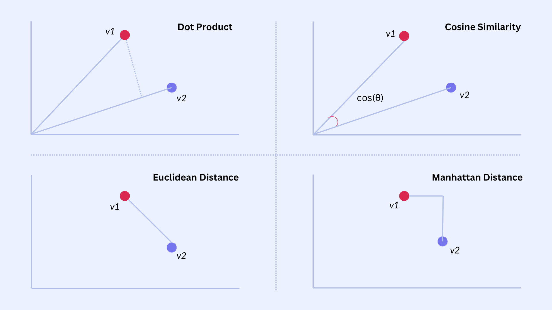
Dot-products compute the similarity of vectors and are closely related to "cosine similarity." In general, distance measures between vectors have many applications in machine learning, since vectors are the fundamental information encoding therein.
Attention
Transformer-based LLMs typically consist of a tall stack of similarly constructed computational layers. Within each layer sits a computation called the "attention mechanism." Pictured below is an analysis of relationships between inputs by calculating the attention pattern. The first LM layer accepts the input prompt, which has often been augmented with RAG search results outside the LM. I mention this nuance because I frequently encounter the misconception that RAG is an integral part of inference. In reality, unless the RAG layer includes metadata in the prompt, the LM has no idea where the RAG content is sourced. Structuring the prompt is the responsibility of the scaffolding around the LM, rather than part of the model itself.
Beyond the first layer, each layer transforms its input sequence (consisting of the prompt tokens/words for the first layer), into the input sequence of the next layer, and so on, until the output flows out of the last layer. The attention layer operates by first multiplying the vector at each input position with learned query, key and value matrices (Wq, Wk, and Wv). That they are "learned" means that these matrices start out randomly initialized, ending up with their final values via the learning algorithms used during training.
The specific Wk, Wq and Wv learned at a given layer in some sense encode a "function" for that layer. In a given layer, the W matrices may learn to process adjectives while other layers may learn to process adverbs, or do arithmetic, or process the word "not," etc. The field of "mechanistic interpretability" studies how models do what they do via their weights and their structure,
During inference, the three W matrices multiply every input vector, yielding a query (Q), key (K) and value (V) vector at each input position. The model then asks "for purposes of this layer, how important is the relationship between every pair of inputs?" by computing every pair's dot product. Each dot product yields a single (scalar) number: When the Q and K vectors are directly aligned, it's larger than when they are not.
Each gray circle below indicates how much the input in that row "attends to" the input in that column: The attention pattern.
Autoregression
Transformer-based LLMs then compute a new "next token." Let's imagine the transformer were processing a sequence consisting of only E1 - E4 so far. To depict E5's production in the above diagram, we would create the E5 column and row, leaving them empty except for the headers.
To fill in the new E5 column, the W matrices are multiplied into the E5 input, yielding Q5, K5 and V5. Running vertically down the new column, the dot product of Q5 with each prior K1 through K4 is computed. The red boxes in the diagram indicate no computation is performed in those boxes when processing text left to right--the new row is left empty except for the E5 box.
The new dot-product "attention pattern" results are then combined with V1-V5 to generate E6, and the process repeats with E6.
KV (but not Q) Cache
The prior K1-K4 and V1-V4 are required to compute the new token, and the current Q5 and V5 are already in memory. When storage is cheaper or faster than compute, these prior K's and V's can be stored in a "KV cache" and re-fetched, rather than be re-computed. On the other hand, the prior Q1-Q4 are no longer needed, as they are relevant only to calculating those prior (no longer needed) attention values.
In other words, the attention pattern diagram above is a historical record of the computations required to generate the complete sequence: The "instant" computation is only in the final column. I mention this because I recall being confused about what exactly the diagram shows when I was first introduced to attention. The two-dimensional grid is often used for two purposes: (1) To show masking, which tokens can attend to which other tokens, effectively displayed by filling only the upper diagonal section and (2) To show what dot products are calculated. Confusingly, only one column at a time is relevant to that second purpose--the last column.
Quadratic in Sequence Length & Cheaper Pre-Fill
In this way, each new token requires multiplying W's into an ever-increasing sequence. For a sequence of length N, the model must do computations proportional to 1+2+…+N because at each step, it must process E1, then E1 and E2, then E1…E3, etc. There is a closed-form formula for that sum:
Thus, looping over ever longer sequences means the cost of computation is quadratic in the sequence length N. LLMs are computationally expensive for long sequences (aka large context windows) for this reason.
This also explains why "pre-fill" tokens are cheaper than generative tokens. The original input prompt requires only a single pass through its N tokens to generate those KVs, and is therefore not quadratic in the pre-fill sequence length.
RoPE
Without positional information, the model would have no way to distinguish the same tokens appearing in different positions: The same W projection matrices are reused at every position. Using the above diagram, the words "fluffy" and "blue" in "a fluffy blue creature" would yield the same K, Q and V irrespective of where in the token sequence they occur. The KQV would not change even if the order of those words were reversed. Not so bad for "fluffy" and "blue," but consider what their relationship should be in "the man hit the ball" vs "the ball hit the man," or when there are 1,000 other words between them.
Clearly, positional information is important to semantic analysis, but the W don't vary with token position. We need something that does.
Rotary Position Embeddings (RoPE) add positional information to the attention calculation by applying a position-dependent rotation to the Q and K vectors, such that their dot product passes that information on to subsequent layers. This happens via the R(x) matrices, where x is the sequence position index, each of which is a linear operator (i.e., a matrix of a specific form). Specifically, these are rotation matrices operating pair-wise on the vector elements. Note this "pair-wise" nature of RoPE when reading about pair-wise dimensionality reduction below.
An important property of these matrix operators is that the subsequent similarity calculation between K and Q (the dot-product) has an output that is itself linear in their positional embedding (i.e., relative position, see red below). In this way, the RoPE information yields an attention result that is dependent on the sequence distance between the subject tokens, but in a way that can be counteracted by the learned W matrices.
Similarity: Nearest-Neighbor and Euclidean Datasets
The dot product is used in other AI-relevant areas, such as information retrieval based on similarity, as in RAG, which fetches documents related to the user's prompt. In the paper, the authors refer to "product quantization" as the term of art used for quantization in the NN literature, and they reference the applicability of TurboQuant to "Euclidean datasets." This is a reference not to the dataset, but to the similarity measure used to characterize the data: A distance metric x-y.
TurboQuant is relevant because when normalizing vectors to ‖x‖ = ‖y‖ = 1, then ‖x − y‖² = ‖x‖² + ‖y‖² − 2⟨x, y⟩ = 2 − 2⟨x, y⟩. For vectors normalized to unit length, the dot product is a proxy for the distance between the vectors. This normalization is mentioned in Section 1.3: "For datasets that do not satisfy this assumption, we can compute and store the L2 norms in floating-point precision, and rescale the dequantized points using these stored norms." The normalization does not limit applicability. However, there is a cost to storing those additional norms:
For each vector, you store b·d bits for the quantized representation plus 32 bits for the norm. The overhead ratio is 32/(b·d). For the DBpedia dataset in the paper with d=1536 at b=2 bits per coordinate, that's 32/(2·1536) ≈ 1% overhead. At d=200 (the GloVe dataset), it's 32/(2·200) = 8% — more noticeable but still modest.
Other metrics are possible:
- Hamming distance counts the number of positions where two binary strings differ. This shows up in DNA sequence comparison, binary feature descriptors in computer vision (like ORB features), and perceptual image hashing.
- Manhattan / L1 distance sums absolute differences: Σ|xᵢ − yᵢ|, for grid navigation or when data are on different scales.
- Hyperbolic distance is for tree-like or hierarchical data because hyperbolic space has exponentially more room as you move outward.
Diving into TurboQuant: Vector Dimensionality
TurboQuant is a combination of several component methods, one of which is motivated by techniques first proposed in the PolarQuant paper. If you learned about TurboQuant via this Google Research page, you would have encountered these statements about PolarQuant:
and
Taken at face value, the first statement says that merely converting to polar coordinates reduces the vector's dimensionality. However, a 3D vector in Cartesian coordinates (x, y, z) has just as many individual coordinates in a spherical coordinate system (r, θ, φ). It is still 3D, just represented differently.
The second statement is similarly unsatisfying. Polar coordinates are by definition a collection of descriptive angles with exactly one radius and the "collection of descriptive angles" would not be smaller than the original when preserving dimensionality, absent additional qualifications.
Therefore, to understand PolarQuant we must go deeper.
Random Preconditioning / Rotation
The TurboQuant paper states "A critical step in the PolarQuant algorithm is random preconditioning of the KV vectors prior to quantization. This involves applying a random projection matrix Π to the embedding vectors before quantizing them…this preconditioning preserves the norms and inner products of … vectors with minimal distortion … [effectively allowing us to treat the vectors as being quantized] from a multivariate normal distribution." In practice, both papersuse random rotations, which preserves norms and inner products exactly; and in the present text, I use these terms interchangeably. PolarQuant's "Fact 3" is most relevant here.
In Section 1.1 of the paper, the authors state "we let the quantizer Q() to be randomized." In the paper, randomness is in the choice of Π, not in repeatedly re-rolling it or randomizing the quantization algorithm itself. You pick one random rotation at initialization, and that single draw is what makes the quantizer "randomized" for analytical purposes. The theoretical guarantees say that for any worst-case input x, the expected distortion over the random draw of Π is bounded. In practice you only draw Π once and it works well because, for high-dimensional vectors, essentially any random rotation does the job — the concentration of measure effects that make each coordinate Beta-distributed and nearly independent kick in reliably for a single draw.
Note that generating Π requires some thought. The TurboQuant paper says Π is generated "by applying QR decomposition on a random matrix with i.i.d Normal entries." For high d, fast structured rotations like random Hadamard transforms are common in practice and preserve the analytical properties approximately. This is hinted at in PolarQuant's reference to random Hadamard matrices.
In section 1.3, the authors state "In high dimensions d, the distribution of each coordinate converges to a Gaussian…" You may wonder, why not in low dimensions? When you take a random rotation Π and compute Πx, each coordinate of the result is a dot product of a row of Π with x. That dot product is a sum of d terms. In high dimensions, you're summing many terms, so the central limit theorem kicks in and the sum looks Gaussian. (Note: The deeper reason is concentration of measure: on a high-dimensional sphere, see Appendix A, most of the surface area is concentrated in a thin band near the equator. If you pick a random point on the sphere in ℝ^d, any single coordinate is very likely to be close to zero with a probability well-approximated by a Gaussian.)
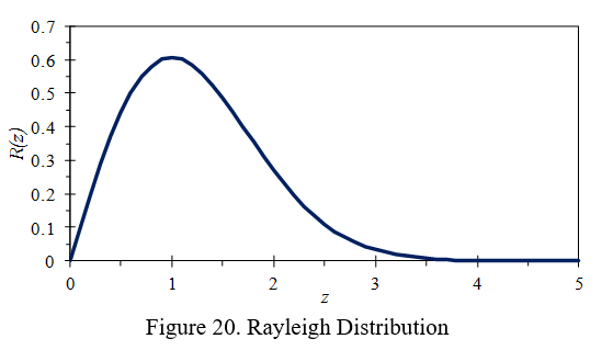
After random preconditioning, the coordinates become approximately i.i.d. Gaussians, which means each pair of coordinates is a 2D Gaussian. A 2D Gaussian in polar form has a Rayleigh-distributed radius (thin shell) and a uniformly distributed angle (convex bodies). Uniform distributions are ideal for fixed-width quantization bins (the angles) and when values are in a thin shell (have a small range), they can be represented with fewer bits (the radii). See Appendix A below for additional information.
Pair-wise Dimensionality Reduction
PolarQuant reduces the dimensionality of each d dimensional vector by grouping pairs of its coordinates, transforming each pair into 2D polar coordinates, producing d/2 such coordinates. So far, there's no change in dimensionality (d/2) * 2 dimensions per pair = d dimensions). The new polar coordinate has an angle and a radius.
PolarQuant quantizes the angle and treats the d/2 new radii as a new d/2 dimensional vector. Next, the d/2 radii of those pairs are treated as if they are cartesian coordinates and those are similarly converted into (d/2)/2 = d/4 pairs of polar coordinates (discarding the prior angles).
The final output consists of a single final radius and a collection of 1, 2, 4, . . . , d/2 angles. Furthermore, "each angle can be quantized independently to minimize the total mean squared error [and jointly] quantizing multiple angle coordinates offers no additional benefit … making [the approach] both computationally efficient and effective."
Thus, PolarQuant quantizes the angles, and stores one radius as a full precision floating point number.
Effect on Size of KV Cache
Per the paper, by storing the centroid (the radius) in the natural floating point format with bF bits while storing the angles, of which there are d-1 (arranged in log d levels), using bQ << bF quantized bits, then the necessary memory is (bF + (d − 1)bQ). The authors state that for Llama-3.1-8B-Instruct with bF = 16, bQ = 3, and d = 128 there is a ~4x reduction in memory.
Note that in practice, PolarQuant recurses for L=4 levels (not all log d levels), which results in 3.875 bits per coordinate in the b=4/2/2/2 schedule on d=128.
How TurboQuant differs
Vector quantization in both PolarQuant and TurboQuant starts by randomly rotating the subject vector. The rotation preserves the relationship between vectors while transforming the properties (distribution) of the vector's coordinates. In dot-product contexts, we also eliminate the dependence on the original directions, making the rotation very useful.
Where PolarQuant works in polar coordinates onto the angles of which the rotation imposes a Gamma distribution, TurboQuant stays in Cartesian coordinates onto which the rotation imposes a Beta distribution (see Appendix B). In common to both techniques is that the random rotation yields coordinates have a distribution with a known analytical form. This means that quantizers can be tuned to those analytical solutions a-priori, without regard to the data.
PolarQuant's recursive polar decomposition requires custom CUDA kernels for the trigonometric encoding/decoding. TurboQuant's simpler Cartesian approach grabs the nearest centroid based on stored indices into precomputed codebooks for the nearest centroid per coordinate, which maps very naturally onto existing GPU primitives (computed in line 6 of Algorithm 1, fetched in line 9). [Note: When I first read the paper, I assumed TurboQuant allowed model computation to be done in compressed space but no, computation is done after de-quantization.]
Diving into TurboQuant: Avoiding Bias
Quantizers that minimize the squared reconstruction error ‖x − x̃‖² make the reconstructed vector x̃ as close as possible to the original. Dprod and/or Dmse from section 1.1 of the paper quantify the "distortion" (reconstruction error) as the variance of those estimates. Bias is about the average of those errors: No bias means those errors average to zero. For an arbitrary vector y, the inner (dot) product of y with the reconstructed vector ⟨y, x̃⟩ may be biased. As you can imagine from the prior discussion of the attention mechanism, such a bias would directly corrupt the model's behavior.
The TurboQuant paper uses QJL, a "sketching" technique (see Appendix D) that eliminates bias. QJL by itself yields significant compression opportunities. As stated in the paper: "When applied across various LLMs and NLP tasks to quantize the KV cache to only 3 bits, QJL demonstrates a more than fivefold reduction in KV cache memory usage without compromising accuracy, all while achieving faster runtime."
The QJL paper also states that "a fundamental concept in numerical linear algebra [is that] applying a Johnson Lindenstrauss (JL) transform, i.e., a random Gaussian projection, to a pair of vectors and then computing the inner product of the projected vectors provides an unbiased and low-distortion estimator for their original inner product." Meanwhile, the TurboQuant paper finds their quantizer is biased despite the random Gaussian projection in it. This is not a contradiction: See Appendix C.
As stated in the TurboQuant paper, after random rotation, "any two distinct coordinates become nearly uncorrelated and, more importantly, almost independent (a deeper result that goes beyond just correlation)." TurboQuant then quantizes each cartesian coordinate using a Max-Lloyd scalar quantizer matched to the coordinates' Beta distribution.
The Max-Lloyd algorithm finds the centroid positions that minimize MSE for a given distribution: First, given the current centroids, set each interval boundary to the midpoint between adjacent centroids (this is the optimal Voronoi partition — each point gets assigned to its nearest centroid). Second, given the current intervals, set each centroid to the conditional mean of the distribution within its interval (this minimizes squared error within each bucket).
Once found, TurboQuant implementations can store codebooks for each desired bit-width permanently, since they depend only on the known Beta distribution, not on any data. This enables fast online quantization.
TurboQuant's Two-Stage Algorithm
Stage 1 applies an MSE-optimal quantizer using a bit-width one less than the target budget. This is the random-rotation-plus-Max-Lloyd quantizer (explained above). This captures the bulk of the vector's information and, crucially, minimizes the L2 norm of the residual r := x − Q⁻¹(Qmse(x)), leaving less work for the second stage.
Stage 2 takes that residual vector r and applies QJL, using the remaining 1 bit in the target budget. Concretely, QJL computes the sign of the inner product between the residual and each of several random Gaussian projection vectors, storing only those sign bits. At query time, the inner product contribution from the residual is estimated from these sign bits using a scaled sum.
The "several random Gaussian projection vectors" are the rows of the random matrix S in the paper. When multiplying S · x, each row of S computes one inner product with x, producing one scalar, which then becomes one sign bit. This produces d sign bits, one per coordinate. [Note: The QJL paper is more general relative to how many sign bits are generated, but in TurboQuant, QJL's m=d.]
Lemma 1
Refer to Appendix A's intuition section, first.
Lemma 1 derives the probability density of a coordinate of a random variable uniformly distributed over the unit hypersphere. The proof is explained via a frequentist relationship between the surface areas and volumes of multi-dimensional "circular" objects: the area of a sphere with radius √(1−x²) in dimension d−1, and the volume of a unit sphere in one higher dimension d, scaled down by 1/√(1−x²).
The √(1−x²) comes from the basic formula for a high-dimensional "circle." The unit sphere equation has the form x₁² + x₂² + … + z² = 1. If we single out one coordinate z, the remaining coordinates must satisfy x₁² + x₂² + … = 1 − z². That's the equation of a (d−2)-sphere whose radius is √(1−z²). In other words, once you fix z, the "slice" of the unit hypersphere at that value of z is itself a lower-dimensional sphere, and its radius is √(1−z²) — shrinking from 1 at z=0 to 0 at the z = ±1.
That radius is what appears throughout the formulas.
The probability density in Lemma 1 gives the probability of finding a uniformly random point on the unit hypersphere at a particular value of one coordinate x. It is the ratio between how much surface area is "at" coordinate value x, divided by the total surface area. The slice of the d-dimensional unit sphere by a hyperplane at coordinate x is another hypersphere with a surface area proportional to (1−x²)^{(d−2)/2}. However, those hypersphere slices are not evenly spaced.
You need a Jacobian (first derivative) correction to convert from "area of the slice" to "density per unit of x." That correction factor is 1/√(1−x²), which comes from the Pythagorean theorem: as you move dx in the coordinate direction, you move a distance ds = dx/√(1−x²) along the sphere's surface; like how arc length on a circle satisfies ds² = dx² + dy² and dy = −x/√(1−x²) dx. In the prior expression y=√(1−x²)
Also note, the paper's actual proof phrasing says fX(x) equals the ratio of the surface area of a sphere with radius √(1−x²) in dimension d−1 to the volume of a unit sphere in dimension d scaled down by 1/√(1−x²): Both the numerator and denominator are surface areas/volumes of standard objects from the same Γ-formula family, which is why so many Γ terms cancel.
QJL Yields an Unbiased Estimator
The QJL algorithm is an efficient, data-oblivious 1-bit quantization approach based on sketching techniques (see Appendix D) that provides unbiased estimates for inner product queries. The key mathematical property is that the QJL estimator satisfies E[⟨y, x̃_qjl⟩] = ⟨y, r⟩ for the residual r. When combined with the first-stage reconstruction, the overall estimator decomposes as:
⟨y, x̃⟩ = ⟨y, x̃_mse⟩ + ⟨y, x̃_qjl⟩
Taking expectations, the proof uses the law of iterated expectation: first conditioning on the MSE reconstruction, then computing the conditional expectation of the QJL correction, which by QJL's unbiasedness property equals the inner product with the true residual.
This chains together to give E[⟨y, x̃⟩] = ⟨y, x⟩, establishing overall unbiasedness.
Distortion Guarantees
In Theorem 2, the paper proves that the b-bit inner product TurboQuant achieves near-optimal distortion for any worst-case vectors x, y with ‖x‖ = 1, with no distributional assumptions on the input. The distortion bound on the inner product error inherits from two sources: the variance of the QJL estimator (which scales with ‖r‖²/d, the MSE of the first stage) and the MSE bound from Theorem 1 applied at bit-width (b−1).
Since the first stage already drove the residual norm close to the information-theoretic minimum, the QJL correction operates on a small residual, keeping the overall variance low. The overall distortion is within a factor of approximately 1.45 of the information-theoretic optimum, which the authors confirm experimentally.
A practical subtlety
One important implementation detail is that you cannot simply add the QJL correction back to the reconstructed vector and store it in the KV cache — doing so injects noise into the vector itself and destroys cosine similarity. The QJL correction must be applied at attention-computation time, inside a fused kernel that uses the two-part representation (the Max-Lloyd indices plus the sign bits and residual norm) directly when computing attention logits. This is why community implementations distinguish between TurboQuant_mse (safe as a drop-in cache replacement) and TurboQuant_prod (which requires a custom attention kernel).
Claude found some references for me:
- "TurboQuant: From Paper to Triton Kernel in One Session" — DEJAN, March 25, 2026. URL: https://dejan.ai/blog/turboquant/
- Kaitchup's "TurboQuant: Finally, Fast and Widely Available Low-Bit KV Cache Quantization?" (March 27, 2026) — explicitly notes "early implementations are converging on the view that the drop-in cache format should usually start with the MSE stage alone, while the QJL residual is more natural when you also own the attention kernel and can consume the two-part representation directly." URL: https://kaitchup.substack.com/p/turboquant-finally-fast-and-widely
- scos-lab/turboquant on GitHub — independent benchmark showing MSE-only outperforms MSE+QJL for attention because softmax amplifies QJL variance more than MSE bias hurts. URL: https://github.com/scos-lab/turboquant
- tonbistudio/turboquant-pytorch on GitHub — reports "0/27 generation tests passed" with QJL, "18/18 passed" without; same root cause. URL: https://github.com/tonbistudio/turboquant-pytorch
Why this matters
The elegance of the construction is that one bit per coordinate is enough to completely eliminate the systematic bias left by the MSE stage, because QJL doesn't need to faithfully reconstruct the residual — it only needs to preserve inner products with arbitrary query vectors in expectation. As one explainer put it, the extra 1-bit stage is not trying to reconstruct every detail of the original vector; it is trying to correct the part that most harms inner-product estimation. Mina This conceptual separation — spend most of your bit budget on MSE-optimal reconstruction, then spend a single bit to "de-bias" the inner product — is what allows TurboQuant to simultaneously achieve near-optimal MSE and unbiased inner product estimation, bridging a gap that neither objective alone could close.
Diving into TurboQuant: Distortion
Yao's minimax principle equates asking:
- "for the best randomized algorithm, what's the worst input?"
- "for the worst distribution over inputs, what's the best deterministic algorithm?"
In the paper, this is used by picking a convenient input distribution (uniform over the unit sphere) to show that even the best deterministic quantizer can't beat (1/d)(1/4^b) distortion on average over that distribution [Note, in the lower bound ||y|| is assumed to be 1 because it's on the unit sphere, but in Theorem 2's upper bound, ||y|| is unconstrained]. Shannon's lower bound comes in because it gives a fundamental limit on how well any compression scheme can do for a given source distribution and bit budget. The chain of reasoning is: best deterministic algorithm against random inputs (bounded by Shannon) = best randomized algorithm against worst-case inputs (what they actually want to bound).
The "2.7" factor in the paper comes from: √3(π/2) · (1/4^b) / (1/4^b) = √3π/2 ≈ 2.7.
Appendix A: High-Dimensional Spaces
Higher Dimensional Intuitions
At dimension d we can consider the embedding of a stable object of one less dimension into that one extra degree of freedom. By "stable object," I mean an object whose lower-dimensional characteristics don't vary with its location in the new dimension. For a given 2D circle on a plane, adding a dimension means being able to translate that circle anywhere along that new 3rd axis. Same circle, different new-dimension coordinate: a cylinder. Adding a 3rd degree of freedom means more than translation — it means allowing for rotation into the new dimension. Rotating a 2D circle around the new dimension from its center yields a 3D sphere.
I think of 4D as a 1D range containing spheres, and thus a 4D sphere as a 3D sphere at a particular point on the 4th axis. We can also invert that relationship, considering a 3D sphere yielding the same scalar value anywhere on its surface. That intuition works for a stable sphere, but now imagine that the 4th coordinate affects the 3D sphere's characteristics. Sliding along the 4th axis causes the 3D sphere to change shape, size, and location.
Regarding the unit hypersphere whose formula is sum(over d coordinates^2) = 1, note that its surface is in fact a d-1 dimensional object, since the constraint removes one degree of freedom. x^2 + y^2 ≤ 1 is a disc, and it's "surface" (the boundary where the it =1) is a circle of one dimension. Put another way, the formula constrains one of the coordinates such that given x there is only one possible y, and thus one dimension.
Vector Things
Here are some fascinating and counterintuitive properties of high-dimensional spaces that come up frequently in theoretical CS and machine learning papers. In all of the below, we discuss n random points (vectors) in d dimensions.
- Nearly all pairs of random vectors are approximately orthogonal. If you draw two vectors independently from a reasonable distribution (e.g., uniform on the unit sphere), their dot-product (similarity) concentrates tightly around zero. This is why random projections preserve structure: They project onto directions that are nearly orthogonal to each other, almost like a true orthonormal basis. This property is frequently leveraged by practitioners.
- Most of the volume of a high-dimensional ball sits near its surface. The fraction of volume within radius 1−ϵ = (1-ϵ)^d. For d=1000 and ϵ=0.01, roughly 99.99% of the volume is in the outermost 1% shell. This is why uniformly sampled points from a high-dimensional ball are at roughly the same distance from the center.
Consequently:
- Random projections preserve geometry (Johnson-Lindenstrauss lemma). Due to 1, you can project n points down to O(log n/ϵ^2) with pairwise distances preserved within a factor of (1±ϵ). Multiplying by a random matrix improves the condition number, spreading the energy of any vector evenly across the basis directions.
- The curse of dimensionality: distances concentrate. Due to 2, as d→∞ the ratio of the points' farthest to nearest distances converges to 1. This means "nearest neighbor" becomes almost meaningless because every point is roughly equidistant from every other point: A fundamental obstacle in high-dimensional search and clustering.
- High-dimensional Gaussians live on a thin shell. Due to 2, when drawing for a multi-dimensional Gaussian the square of their magnitudes (||X||^2) concentrates around d with standard deviation O(sqrt(d)). Put another way, every sample from a high-dimensional Gaussian sits on a sphere of radius ≈ sqrt(d). This explains the sqrt() normalization terms you see in the denominator of many equations.
- Convex bodies in high dimensions are surprisingly "round" (Milman's theorem). Every convex body has a roughly sqrt(d) dimensional central section that is approximately an ellipsoid. This implies any Lipschitz function (who's output does not change too fast with input changes) is nearly constant. This is why randomized algorithms over convex sets behave so predictably.
- Exponentially many nearly orthogonal vectors can coexist. Due to 1, you can pack exp(cd) vectors that are all pairwise within angle 90°±ϵ for small ϵ (where c is some constant related to ϵ). This exponential packing capacity is what makes compressed sensing, random codes, and dimensionality reduction work — you have far more "almost independent" directions available than the dimension would naively suggest.
These facts are all interconnected through the concentration of measure phenomenon: in high dimensions, random quantities tend to be very close to their expectations, and this predictability is what allows randomized algorithms to offer strong guarantees.
Appendix B: Named Distributions & The Gamma Function
In PolarQuant, we encounter Rayleigh and Gamma distributions. In TurboQuant, we encounter the Beta distribution. Both papers consider distributions related to a point uniformly distributed on the unit sphere. Where PolarQuant asks about the distribution of the radius coordinate of such a point, TurboQuant asks about a single cartesian coordinate of that point.
These two settings are related by a classical connection. If you take a d-dimensional Gaussian vector and normalize it to unit length, you get a uniform point on the unit ball. Each coordinate of that uniform point follows the distribution given in TurboQuant's Lemma 1: A scaled and shifted Beta distribution. By contrast, the radii in PolarQuant follow a Rayleigh distribution.
There is a connection between various named distributions:
Gamma/Chi: Given a d-dimensional Gaussian vector, what is the distribution of its length? This is the radial question.
Rayleigh: The Gamma/Chi answer for d=2 (i.e., in two dimensions).
Beta: What is the distribution of a single Cartesian coordinate? This is the projection question in TurboQuant because it quantizes each coordinate directly.
The Gamma Function
The Gamma function is a continuous version of the discrete factorial.
It shows up in the papers in many places because the surface area of a sphere in d dimensions is derived by integrating over angles, which produces integrals of sin^k(θ) for various powers k. These integrals evaluate to ratios of Gamma functions (since ∫sin^k(θ)dθ is a Beta function integral, and the Beta function is defined in terms of Gamma functions). So the Gamma function shows up because it's what you get when you accumulate the results of integrating over each angular coordinate one at a time.
More intuitively, in low dimensions, sphere surface areas involve integer factorials: the circumference of a circle is 2π, the surface area of a 3-sphere is 4π, and the pattern involves factors like 2πr multiplied by factorial-like terms from repeated integration. But the sphere area formula needs to work for all dimensions, and the recursive structure (the area in dimension d depends on the area in dimension d−1) involves dividing by quantities that are half-integers when d is odd. You can't write (3/2)! using ordinary factorials, but Γ(5/2) handles it naturally. So the Gamma function appears because the dimension d can be any integer, which means the formulas inevitably pass through half-integer "factorials" that only the Gamma function can express.
Appendix C: Johnson- Lindenstrauss (JL) transforms vs Random Rotations
A JL transform in the classical sense is a random projection from ℝ^d to ℝ^m where typically m < d. An outcome is dimensionality reduction while approximately preserving inner products and distances. The JL lemma guarantees that with m = O(ε⁻² log n) dimensions, all pairwise distances among n points are preserved up to a (1 ± ε) factor. This Lemma is invoked in the PolarQuant paper.
TurboQuant and PolarQuant use square d × d random orthogonal matrices, rotations that map ℝ^d to ℝ^d with no dimensionality reduction. Inner products and norms are preserved exactly. The purpose is to randomizing coordinates so that they can derive analytical statistics to drive online algorithms.
Appendix D: A note about terminology ("online" "offline" "residual" "sketching")
Canonically, an "online" algorithm processes its input piece-by-piece as the input arrives, without having the entire input available from the start. In contrast, an offline algorithm is given all the data up front. In an offline algorithm, data that arrive later can influence results from earlier data, for example when we use a statistic calculated from the complete dataset to make calculations using a subset of the data.
In a quantization context, "online" means the quantizer can be fully specified before seeing any data: Each new vector can be quantized immediately as it arrives, with no dependence on past or future vectors. When the data have known analytical distributions, the statistics of that distribution are (by definition) known before the data arrive and can be used to quantize those data as they arrive.
"Offline" means the quantizer needs a pass over the dataset first (e.g., running k-means to learn codebooks): In general, offline (data-dependent) methods often require heavy preprocessing and learning to adapt the quantization map to the data, making them unsuitable for dynamic data scenarios.
In these papers "residual" means the difference between the original vector and the reconstructed vector. If you're learning about LLMs you've also heard this term in the phrase "residual stream," which comes from A Mathematical Framework for Transformer Circuits. There, it refers to the residual connection (also called a skip connection): The long vertical line with the (+) on the left of this diagram:
In transformers, the output of a layer is added back to its input before passing to the next layer. In that sense, the output of a layer is a residual in the same sense as in the quantization context because it's what's added to get from where you are to where you want to be. The quantization error similarly gets you back to the original vector, when adding back to the quantized version.
In computer science and applied mathematics, "sketching" refers to a family of randomized algorithms that compress data while preserving important properties. The term comes from the idea of creating a compact "sketch" of the data that can be used for approximate computations.
Appendix E: Yao's Minimax Principle
Appendix F: Differential Entropy & Mutual Information
Lemma 2 contains two quantities: h(x), the differential entropy of the source, and B, which is a bit budget tied to mutual information I(x; y) between the original and reconstructed vectors. For a discrete random variable, entropy H(X) measures the average number of bits you need to describe a sample. High entropy means high uncertainty, low entropy means the variable is concentrated and predictable. A fair coin has H = 1 bit; a heavily biased coin has H close to 0 (and cannot be negative).
The continuous version of discrete entropy applied to a probability density p(x) is h(x) = −∫ p(x) log p(x) dx (and can be negative). It is not an absolute measure of information and h(x) = 3 should not be read as 3 bits of information. Instead, it means something more like "x typically takes up a log-volume of 3," (in log-volume units of x). To make it meaningful, we take differences between h(x) and some other h(y), which tells us how much more spread out x is, and is why it shows up in the Shannon Lower Bound paired with B.
Mutual information I(X;Y) = H(X) - H(X | Y) measures how much knowing either or y reduces your uncertainty about the other variable (it's symmetric). If they are independent, I(X;Y)=0. If you encode X into B bits, and then decode that into a value we'll call Y, then we expect I(X;Y) < B. You can't get more bits out than the width of your communication channel! That's what makes the Shannon Lower Bound a fundamental lower bound.
Int TurboQuant Section 2.1: Mutual information combined with the uniform on-sphere distribution gives us the 2.7 lower bound.
In TurboQuant Section 3.1: The random rotation preserves all properties. The information content is preserved.
In PolarQuant 2.2 (footnote): Per the intuition I provided in Appendix A, the "concentration of measure," is about high-dimensional uniform distributions concentrating most of their entropy (information) in tiny regions i.e. the sphere shell and the equatorial band, where things look like Gaussians and mutual information collapses to zero.
See:
1. 3Blue1Brown — "Solving Wordle using information theory" (Grant Sanderson, 2022)
- Video: https://www.youtube.com/watch?v=v68zYyaEmEA
- Companion lesson page: https://www.3blue1brown.com/lessons/wordle
2. Christopher Olah — "Visual Information Theory" (colah.github.io, 2015)